%config IPCompleter.use_jedi = False
%load_ext autoreload
%autoreload 2
%matplotlib inline
import matplotlib as mpl
mpl.rcParams['figure.dpi'] = 300
import pandas as pd
import numpy as np
from scipy import sparse
import os
import plotly.express as px
import seaborn as sns
from functions import *
os.chdir("/Users/schilder/Desktop/AD_CVD_genetics/")
intro()
DEGAS = np.load("./raw_data/DEGAS/dev_allNonMHC_z_center_p0001_100PCs_20180129.npz", allow_pickle=True)
# list(DEGAS.keys())
for x in list(DEGAS.keys()):
print(x)
try:
print(DEGAS[x].shape)
except:
print(len(DEGAS[x]))
# "loading_phe","contribution_phe","eigen_phe","cos_phe"
loading_phe = pd.DataFrame(data=DEGAS["contribution_phe"],
columns=["PC"+str(x+1) for x in range(0,DEGAS["contribution_phe"].shape[1])],
index=DEGAS["label_phe"])
loading_phe
Import metdata
meta = pd.read_excel("raw_data/DEGAS/41467_2019_11953_MOESM5_ESM.xlsx")
meta = meta.merge(pd.DataFrame({"label_phe":DEGAS["label_phe"], "label_phe_code":DEGAS["label_phe_code"]}), on="label_phe_code")
## Assign AD/CVD status
meta["CVD"] = meta["label_phe"].str.lower().str.contains("cardiom|cardia|heart|vascular|atrial|atrium")
meta["AD"] = meta["label_phe"].str.lower().str.contains("alzheimer")
conditions = [
(meta['AD'] == True),
(meta['CVD'] == True)
]
values = ['AD','CVD']
meta['AD_CVD'] = np.select(conditions, values)
AD_terms = meta.loc[meta["AD"],:].label_phe.tolist()
CVD_terms = meta.loc[meta["CVD"],:].label_phe.tolist()
AD_CVD_terms = AD_terms + CVD_terms
# Sample size
meta["N_cases"] = np.log1p(meta["Number of cases"])
meta.loc[meta["AD_CVD"].isin(["AD","CVD"]),:]
PCA
The top 2 PCs don't really generate identifiable clusters beyond Physical Measurement (mostly related to adiposity/BMI) and others.
pca_annot = loading_phe.merge(meta, left_index=True, right_on="label_phe")
fig = px.scatter(pca_annot, x="PC1", y="PC2", #height=400,
log_x=True, log_y=True,
opacity=.8, color="Category",#"AD_CVD",
hover_data=["label_phe","AD_CVD","Number of cases"])
fig.update_traces(marker=dict(size=10))
fig.show()
UMAP
UMAP (using the PCs as input) gives a much better visual representation of the data. But it's unclear how many of the 100 PCs to use. So we iterate running UMAP with an increasing number of PCs.
umap_df_list = [get_umap(loading_phe, meta, n_dims=x, merging_var="label_phe") for x in [2,3,4,10,20,40,60,80,100]]
umap_df = pd.concat(umap_df_list)
umap_df
2D UMAP
def animated_scatter(umap_df,
threeD=True,
x="UMAP1", y="UMAP2", z="UMAP3",
animation_frame="n_dims",
animation_group="label_phe",
size="N_cases", size_max=10, height=600,
opacity=.8, color="Category",
hover_data=["label_phe","AD_CVD","Number of cases"],
duration=2000,
renderer="notebook",
show_plot=True):
import plotly.express as px
if threeD:
fig = px.scatter_3d(umap_df, x=x, y=y, z=z,
animation_frame=animation_frame,
animation_group=animation_group,
size=size, size_max=size_max,height=height,
title=f'{umap_df[animation_frame].unique()[0]} input dimensions',
opacity=opacity, color=color,
hover_data=hover_data)
else:
fig = px.scatter(umap_df, x=x, y=y,
animation_frame=animation_frame,
animation_group=animation_group,
size=size, size_max=size_max,height=height,
title=f'{umap_df[animation_frame].unique()[0]} input dimensions',
opacity=opacity, color=color,
hover_data=hover_data)
for button in fig.layout.updatemenus[0].buttons:
button['args'][1]['frame']['redraw'] = True
for k in range(len(fig.frames)):
n_dims = umap_df["n_dims"].unique()[k]
fig.frames[k]['layout'].update(title_text=f'{n_dims} input dimensions')
fig.update_traces(hoverlabel = dict(font=dict(color='white')))
fig.layout.updatemenus[0].buttons[0].args[1]["frame"]["duration"] = duration
# Hover modes: https://plotly.com/python/hover-text-and-formatting/
# fig.update_traces(hovertemplate=None)
# fig.update_layout(hovermode="x unified")
if show_plot:
fig.show(renderer="notebook")
return fig
fig = animated_scatter(umap_df, x="UMAP1", y="UMAP2",
threeD=False,
animation_frame="n_dims", animation_group="label_phe",
size="N_cases", size_max=5,height=600,
opacity=.8, color="Category",
hover_data=["label_phe","AD_CVD","Number of cases"])
3D UMAP
fig = animated_scatter(umap_df, x="UMAP1", y="UMAP2",
animation_frame="n_dims", animation_group="label_phe",
size="N_cases", size_max=15,height=600,
opacity=.8, color="Category",
hover_data=["label_phe","AD_CVD","Number of cases"])
Identify overlapping AD-CVD component(s)
Get top PCs
- Get the PCs with the top N highest or lowest mean loadings for each of the phenotype groups (AD and CVD).
- Then, find the intersect between each of the highest/lowest PC pairs across groups. This high/low pairing ensures the phenotype groups aren't loaded in the opposite directions.
top_PCs = get_topPCs(loading_phe, meta, terms1=AD_terms, terms2=CVD_terms, top_n=10)
top_PCs
Heatmaps
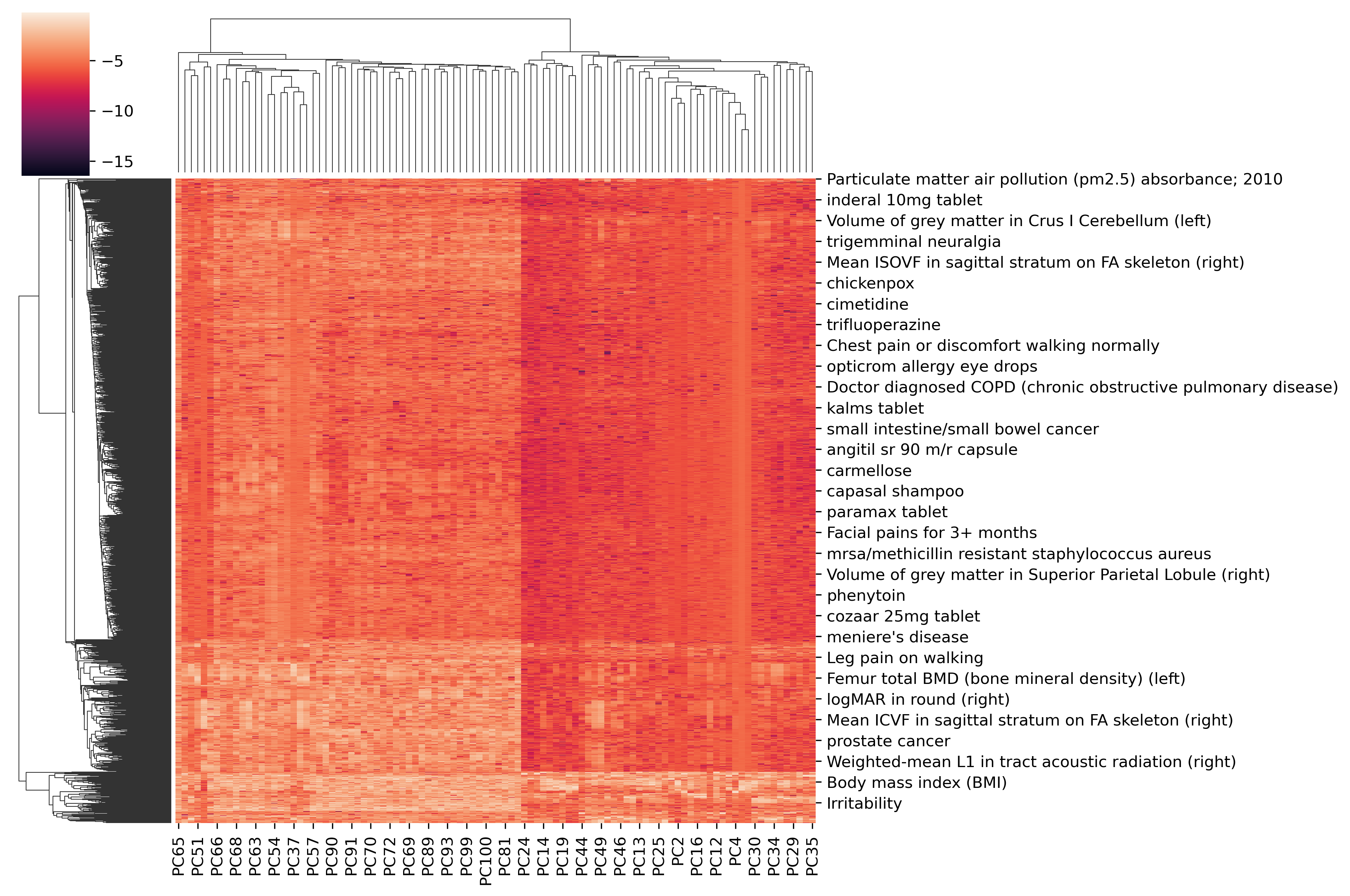
All phenotypes x all PCs
fig = sns.clustermap(np.log10(loading_phe), figsize=(12,8))
Phenotypes x phenotypes
## ALL phenotypes x all phenotypes
## Takes a very long time to run
# corr_mat = loading_phe.T.corr()
# fig = sns.clustermap(corr_mat, figsize=(20,20))
corr_mat = loading_phe.loc[AD_CVD_terms,:].T.corr()
# corr_mat.to_csv("processed_data/DEGAS/all_traits.corr.csv.gz")
corr_mat.to_csv("processed_data/DEGAS/AD_CVD.corr.csv.gz")
# https://docs.bokeh.org/en/latest/docs/user_guide/jupyter.html#userguide-jupyter-notebook
from bokehheat import heat
from bokeh.palettes import Reds9, RdBu11, YlGn8, Colorblind8
from bokeh.io import output_notebook
from bokeh.plotting import figure, show
output_notebook()
s_filename="processed_data/DEGAS/AD_CVD.clustergram.html"
o_clustermap, ls_xaxis, ls_yaxis = heat.clustermap(
df_matrix = corr_mat,
ls_color_palette = Reds9,
r_low = 0,
r_high = 1,
# s_z = "log2",
b_ydendo = True,
b_xdendo = True,
s_filetitel="Phenotype x phenotype correlation",
s_filename=s_filename
)
# show(o_clustermap)
from IPython.display import Markdown as md
md("[Clustergram link]({})".format("https://neurogenomics.github.io/AD_CVD_genetics/"+s_filename))
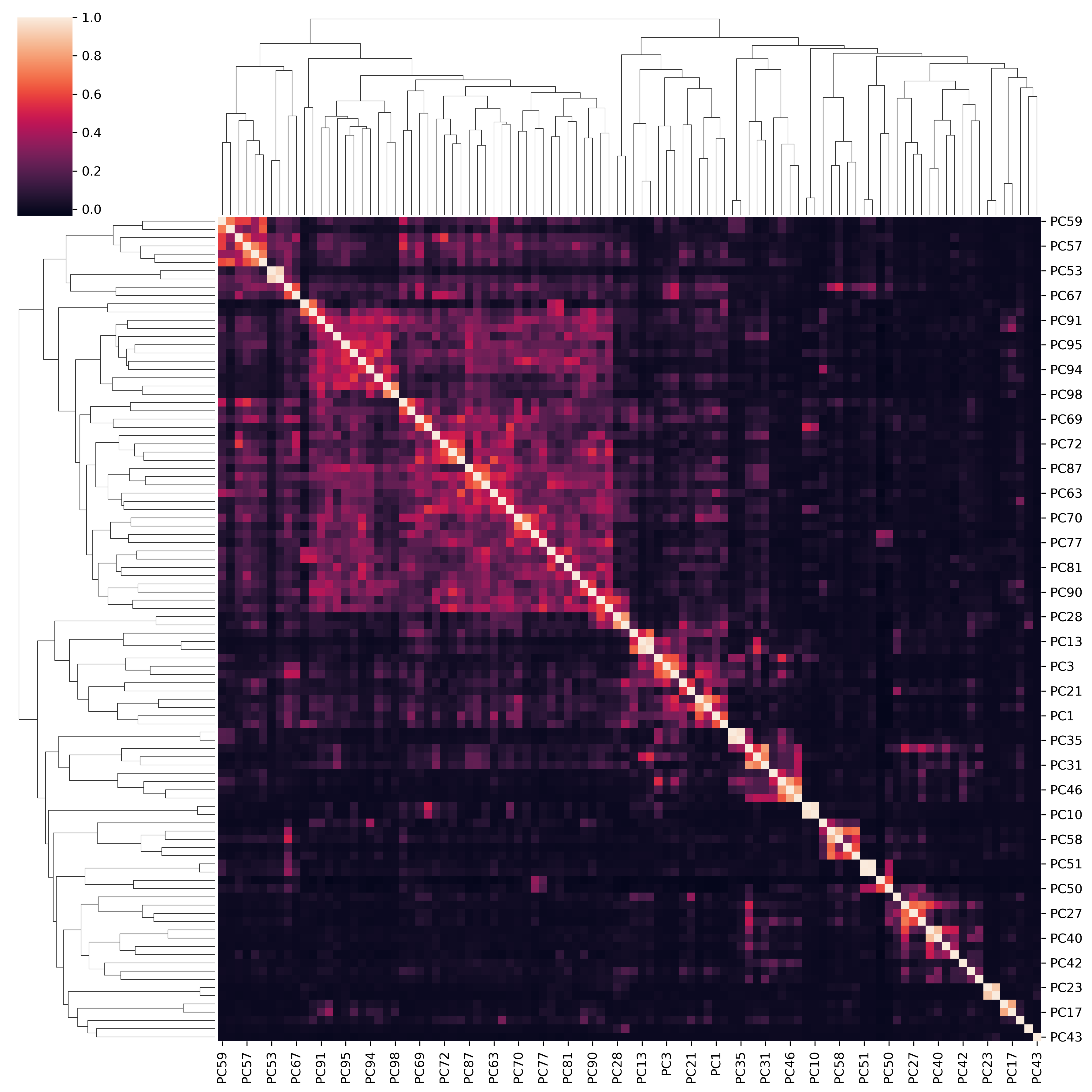
All PCs vs. all PCs
corr_mat_PC = loading_phe.corr()
fig = sns.clustermap(corr_mat_PC, figsize=(12,12))
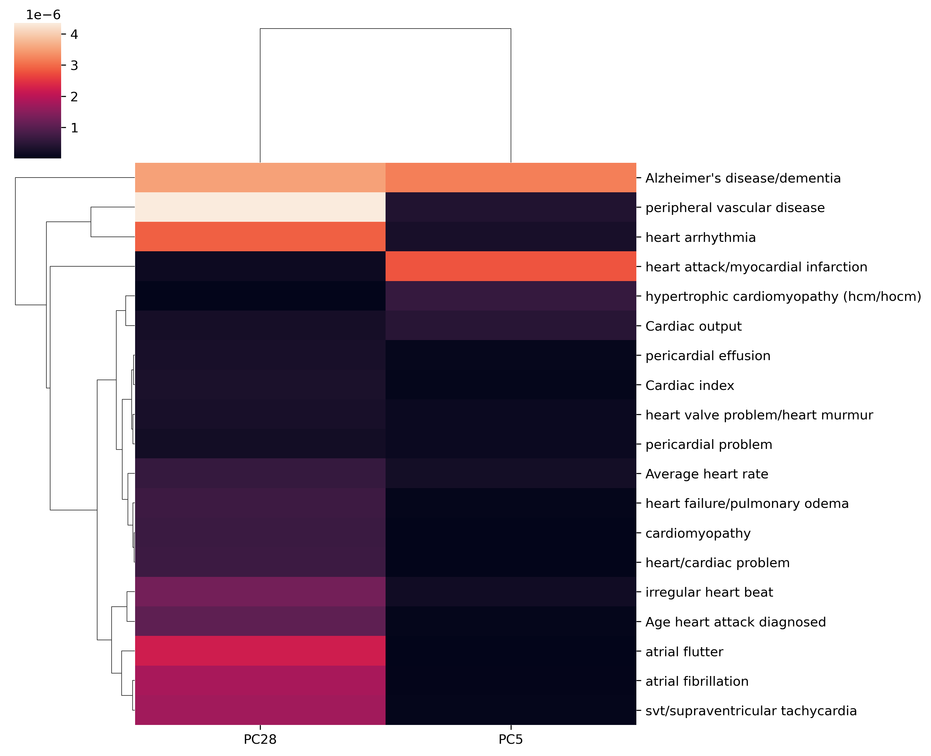
AD/CVD phenotypes x top PCS
# https://plotly.com/python-api-reference/generated/plotly.express.imshow
px.imshow(loading_phe.loc[AD_terms+CVD_terms, top_PCs], aspect=.5)
sns.clustermap(loading_phe.loc[AD_terms+CVD_terms,top_PCs], figsize=(10,8))
Identify variants
variants = pd.DataFrame(DEGAS["contribution_var"],
index=DEGAS["label_var"],
columns=["PC"+str(x+1) for x in range(0,DEGAS["contribution_var"].shape[1])])
print(variants.shape)
variants.head()
sorted_variants = get_top_loadings(loadings=variants, top_PCs=top_PCs, top_n=10, var_name="variant")
sorted_variants
save_table(df=variants.loc[:,top_PCs], df_path= "processed_data/DEGAS/AD_CVD.all_variants.csv.gz")
save_table(df=sorted_variants, df_path= "processed_data/DEGAS/AD_CVD.variants.csv.gz")
Identify genes
genes = pd.DataFrame(DEGAS["contribution_gene"],
index=DEGAS["label_gene"],
columns=["PC"+str(x+1) for x in range(0,DEGAS["contribution_gene"].shape[1])])
# Remove variants that are in this dataframe for some reason
genes = genes.loc[~genes.index.isin(variants.index),:]
print(genes.shape)
genes.head()
sorted_genes = get_top_loadings(loadings=genes, top_PCs=top_PCs, top_n=10, var_name="gene")
sorted_genes
"IRX3" in sorted_genes.gene
Genes of particular interest
FTO: FTO affects obesity through regulation of hypothalamic neurons (and thus eatin behaviour), though this is achieved through its regulation of IRX3, which is a less direct mechanism than once thought. In relaton to AD:
"Recent studies revealed that carriers of common FTO gene polymorphisms show both a reduction in frontal lobe volume of the brain[39] and an impaired verbal fluency performance.[40] Fittingly, a population-based study from Sweden found that carriers of the FTO rs9939609 A allele have an increased risk for incident Alzheimer disease.[41]" -Wikipedia
FANCA: gene named after Fanconi anemia, a rare blood disorder.
save_table(df=genes.loc[:,top_PCs], df_path= "processed_data/DEGAS/AD_CVD.all_genes.csv.gz")
save_table(df=sorted_genes, df_path= "processed_data/DEGAS/AD_CVD.genes.csv.gz")
Determine outlier genes
- Find the genes that signficantly more associated with these PCs than other PCs.
- sklearn has a number of outlier/anomaly detection tools to do this. However these methods are all designed to make predictions from a matrix of the same size as the one you trained on, unless you fit_predict on the several PCs of interest directly. At which point, you're basically just fiddling with the hyperparameters to get the desired number of genes (very similar to the simple table sorting method).
- gene-outlier-detection is explicitly designed for genes.
from sklearn.neighbors import LocalOutlierFactor
X = genes.loc[:,~genes.columns.isin(top_PCs)]
y = genes.loc[:,top_PCs]
# use fit_predict to compute the predicted labels of the training samples
# (when LOF is used for outlier detection, the estimator has no predict,
# decision_function and score_samples methods)
clf = LocalOutlierFactor(n_neighbors=20, contamination=0.001)
y_pred = clf.fit_predict(y)
y.index[y_pred==-1]
### NOTE: have to add --ExecutePreprocessor.timeout=180 to avoid timeout.
# !jupyter nbconvert --to html_toc --ExecutePreprocessor.timeout=180 --execute code/DeGAs.ipynb