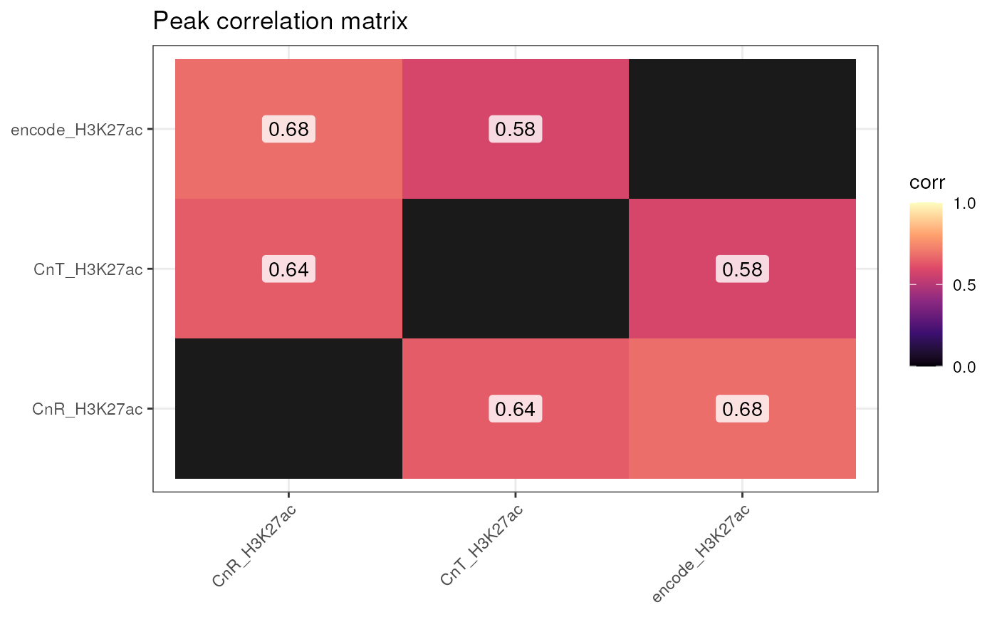
Plot correlation by binning genome and measuring correlation of peak quantile ranking. This ranking is based on p-value or other peak intensity measure dependent on the peak calling approach.
plot_corr(
  peakfiles,
  reference = NULL,
  genome_build,
  bin_size = 5000,
  keep_chr = NULL,
  drop_empty_chr = FALSE,
  method = "spearman",
  intensity_cols = c("total_signal", "qValue", "Peak Score", "score"),
  interact = FALSE,
  draw_cellnote = TRUE,
  fill_diag = NA,
  workers = check_workers(),
  show_plot = TRUE,
  save_path = tempfile(fileext = ".corr.csv.gz")
)
Arguments
- peakfiles
A list of peak files as GRanges object and/or as paths to BED files. If paths are provided, EpiCompare imports the file as GRanges object. EpiCompare also accepts a list containing a mix of GRanges objects and paths.Files must be listed and named using
list(). E.g.list("name1"=file1, "name2"=file2). If no names are specified, default file names will be assigned.- reference
A named list containing reference peak file(s) as GRanges object. Please ensure that the reference file is listed and named i.e.
list("reference_name" = reference_peak). If more than one reference is specified, individual reports for each reference will be generated. However, please note that specifying more than one reference can take awhile. If a reference is specified, it enables two analyses: (1) plot showing statistical significance of overlapping/non-overlapping peaks; and (2) ChromHMM of overlapping/non-overlapping peaks.- genome_build
The build of **all** peak and reference files to calculate the correlation matrix on. If all peak and reference files are not of the same build use liftover_grlist to convert them all before running. Genome build should be one of hg19, hg38, mm9, mm10.
- bin_size
Default of 100. Base-pair size of the bins created to measure correlation. Use smaller value for higher resolution but longer run time and larger memory usage.
- keep_chr
Which chromosomes to keep.
- drop_empty_chr
Drop chromosomes that are not present in any of the
peakfiles(default:FALSE).- method
Default spearman (i.e. non-parametric). A character string indicating which correlation coefficient (or covariance) is to be computed. One of "pearson", "kendall", or "spearman": can be abbreviated.
- intensity_cols
Depending on which columns are present, this value will be used to get quantiles and ultimately calculate the correlations:
"total_signal" : Used by the peak calling software SEACR. NOTE: Another SEACR column (e.g. "max_signal") can be used together or instead of "total_signal".
"qValue"Used by the peak calling software MACS2/3. Should contain the negative log of the p-values after multiple testing correction.
"Peak Score" : Used by the peak calling software HOMER.
- interact
Default TRUE. By default heatmap is interactive. If FALSE, heatmap is static.
- draw_cellnote
Draw the numeric values within each heatmap cell.
- fill_diag
Fill the diagonal of the overlap matrix.
- workers
Number of threads to parallelize across.
- show_plot
Show the plot.
- save_path
Path to save a table of correlation results to.
Value
list with correlation plot (corr_plot) and correlation matrix (data)
Examples
data("CnR_H3K27ac")
data("CnT_H3K27ac")
data("encode_H3K27ac")
peakfiles <- list(CnR_H3K27ac=CnR_H3K27ac, CnT_H3K27ac=CnT_H3K27ac)
reference <- list("encode_H3K27ac"=encode_H3K27ac)
## Increasing bin_size for speed here,
## but lower values will give more precise results (and lower correlations)
cp <- plot_corr(peakfiles = peakfiles,
                reference = reference,
                genome_build = "hg19",
                bin_size = 5000,
                workers = 1)
#> Standardising peak files in 647,114 bins of 5,000 bp.
#> Merging data into matrix.
#> Binned matrix size: 647,114 x 3
#> Matrix sparsity: 0.996
#> Calculating correlation matrix.
#> Done computing correlations in 3 seconds.
#> Saving correlation results ==> /tmp/RtmpYYVLJl/file4b42472cb77d.corr.csv.gz
