Functions to plot data.
plot_clinvar(
  hits,
  x = "region",
  y = "N",
  fill = "Type",
  rows = "ClinSigSimple",
  by = c("build", x, fill, rows)
)

plot_ggnetwork(
  g,
  colour_var = "x",
  size_var = colour_var,
  label_var = "name",
  hoverbox_column = "hover",
  interactive = TRUE,
  show_plot = TRUE,
  ...
)

plot_graph_3d(
  g,
  layout_func = igraph::layout.fruchterman.reingold,
  id_var = "name",
  node_color_var = "ancestor_name",
  edge_color_var = "zend",
  text_color_var = node_color_var,
  node_symbol_var = "ancestor_name",
  node_palette = pals::kovesi.cyclic_mrybm_35_75_c68_s25,
  edge_palette = pals::kovesi.cyclic_mrybm_35_75_c68_s25,
  node_opacity = 0.75,
  edge_opacity = 0.5,
  kde_palette = pals::gnuplot,
  add_kde = TRUE,
  extend_kde = 1.5,
  bg_color = kde_palette(6)[1],
  add_labels = FALSE,
  keep_grid = FALSE,
  aspectmode = "cube",
  hover_width = 100,
  label_width = 100,
  seed = 2023,
  showlegend = TRUE,
  show_plot = TRUE,
  save_path = tempfile(fileext = "plot_graph_3d.html"),
  verbose = TRUE
)

plot_ontology(
  ont,
  terms = NULL,
  types = c("circular", "graphviz", "tidygraph", "visnetwork"),
  ...
)

plot_ontology_circular(ont, ...)

plot_ontology_graphviz(ont, ...)

plot_ontology_heatmap(
  ont,
  annot = data.table::data.table(as.data.frame(ont@elementMetadata)),
  X = ontology_to(ont, to = "similarity"),
  fontsize = ont@n_terms * 4e-04,
  row_labels = ont@terms,
  column_labels = row_labels,
  name = NULL,
  row_side_vars = c("ancestor_name"),
  col_side_vars = c("IC", "depth", "n_children", "n_offspring", "n_connected_leaves"),
  col = pals::gnuplot(),
  show_plot = TRUE,
  save_path = tempfile(fileext = "plot_ontology_heatmap.pdf"),
  height = 12,
  width = height * 1.1,
  seed = 2023,
  types = c("heatmaply", "ComplexHeatmap")[2],
  ...
)

plot_ontology_tidygraph(ont, ...)

plot_ontology_visnetwork(ont, ...)

plot_save(plt, save_path = save_path, width = NULL, height = width)

plot_upheno_heatmap(
  plot_dat,
  lvl = 10,
  ont = get_ontology("upheno", lvl = lvl),
  hpo_ids = NULL,
  value.var = c("phenotype_genotype_score", "prop_intersect", "equivalence_score",
    "subclass_score"),
  name = value.var[1],
  min_rowsums = NULL,
  cluster_from_ontology = FALSE,
  save_dir = tempdir(),
  height = 15,
  width = 10
)Arguments
- g
ggnetwork object (or an igraph/tbl_graph to be converted to ggnetwork format).
- colour_var
Column to color nodes by.
- size_var
Column to scale node size by.
- label_var
Column containing the label for each node in a graph (e.g. "hpo_name").
- interactive
Make the plot interactive.
- show_plot
Print the plot after it's been generated.
- ...
Arguments passed on to
ggplot2::aes,simona::dag_circular_viz,simona::dag_graphviz,base::plot,simona::dag_graphvizdagAn
ontology_Dagobject.highlightA vector of terms to be highlighted on the DAG.
startStart of the circle, measured in degree.
endEnd of the circle, measured in degree.
partition_by_levelIf
node_colis not set, users can cut the DAG into clusters with different node colors. The partitioning is applied bypartition_by_level().partition_by_sizeSimilar as
partition_by_level, but the partitioning is applied bypartition_by_size().node_colColors of nodes. If the value is a vector, the order should correspond to terms in
dag_all_terms().node_transparencyTransparency of nodes. The same format as
node_col.node_sizeSize of nodes. The same format as
node_col.edge_colA named vector where names correspond to relation types.
edge_transparencyA named vector where names correspond to relation types.
legend_labels_fromIf partitioning is applied on the DAG, a legend is generated showing different top terms. By default, the legend labels are the term IDs. If there are additionally column stored in the meta data frame of the DAG object, the column name can be set here to replace the term IDs as legend labels.
legend_labels_max_widthMaximal width of legend labels measured by the number of characters per line. Labels are wrapped into multiple lines if the widths exceed it.
other_legendsA list of legends generated by
ComplexHeatmap::Legend().use_rasterWhether to first write the circular image into a temporary png file, then add to the plot as a raster object?
newpageWhether call
grid::grid.newpage()to create a new plot?node_paramA list of parameters. Each parameter has the same format. The value can be a single scalar, a full length vector with the same order as in
dag_all_terms(), or a named vector that contains a subset of terms that need to be customized. The full set of parameters can be found at https://graphviz.org/docs/nodes/.edge_paramA list of parameters. Each parameter has the same format. The value can be a single scalar, or a named vector that contains a subset of terms that need to be customized. The full set of parameters can be found at https://graphviz.org/docs/edges/. If the parameter is set to a named vector, it can be named by relation types
c("is_a" = ...), or directly relationsc("a -> b" = ...). Please see the vignette for details.rankdirThe direction of the layout. Only four values are allowed:
"TB","LR","BT"and"RL".xthe coordinates of points in the plot. Alternatively, a single plotting structure, function or any R object with a
plotmethod can be provided.ythe y coordinates of points in the plot, optional if
xis an appropriate structure.
- layout_func
Layout function for the graph.
- node_color_var
Variable in the vertex metadata to color nodes by.
- edge_color_var
Variable in the edge metadata to color edges by.
- text_color_var
Variable in the node metadata to color text by.
- node_symbol_var
Variable in the vertex metadata to shape nodes by.
- node_palette
Color palette function for the nodes/points.
- edge_palette
Color palette function for the edges/lines.
- node_opacity
Node opacity.
- edge_opacity
Edge opacity.
- kde_palette
Color palette function for the KDE plot.
- add_kde
Add a kernel density estimation (KDE) plot below the 3D scatter plot (i.e. the "mountains" beneath the points).
- extend_kde
Extend the area that the KDE plot covers.
- bg_color
Plot background color.
- add_labels
Add phenotype name labels to each point.
- keep_grid
Keep all grid lines and axis labels.
- aspectmode
The proportions of the 3D plot. See the plotly documentation site for details.
- hover_width
Maximum width of the hover text.
- label_width
Maximum width of the label text.
- seed
Set the seed for reproducible clustering.
- showlegend
Show node fill legend.
- save_path
Path to save interactive plot to as a self-contained HTML file.
- verbose
Print messages.
- ont
An ontology of class ontology_DAG.
- terms
A vector of ontology term IDs.
- types
Types of graph to produce. Can be one or more.
- fontsize
Axis labels font size.
- row_labels
Optional row labels which are put as row names in the heatmap.
- column_labels
Optional column labels which are put as column names in the heatmap.
- name
Name of the heatmap. By default the heatmap name is used as the title of the heatmap legend.
- row_side_vars
Variables to include in row-side metadata annotations.
- col_side_vars
Variables to include in column-side metadata annotations.
- col
A vector of colors if the color mapping is discrete or a color mapping function if the matrix is continuous numbers (should be generated by
colorRamp2). If the matrix is continuous, the value can also be a vector of colors so that colors can be interpolated. Pass toColorMapping. For more details and examples, please refer to https://jokergoo.github.io/ComplexHeatmap-reference/book/a-single-heatmap.html#colors .- height
Height of the heatmap body.
- width
Width of the heatmap body.
- save_dir
Directory to save a file to.
Value
A named list containing the plot and the data.
A 3D interactive plotly object.
Null
Null
Plot
Null
Null
Functions
plot_clinvar(): plot_ Plot mapped variant annotations.plot_ggnetwork(): plot_ Plot a ggnetwork.plot_graph_3d(): plot_ 3D networkPlot a subset of the HPO as a 3D network.
plot_ontology(): plot_plot_ontology_circular(): plot_plot_ontology_graphviz(): plot_ Plot ontology: graphvizMake a circular plot of an ontology.
plot_ontology_heatmap(): plot_ Plot heatmapPlot a phenotype x phenotype correlation matrix based on genetic overlap.
plot_ontology_tidygraph(): plot_plot_ontology_visnetwork(): plot_plot_save(): plot_ Save a plot using ggsave, grDevices, or visSave.plot_upheno_heatmap(): plot_
Examples
ont <- get_ontology(terms=10)
#> Using cached ontology file (1/1):
#> /github/home/.cache/R/KGExplorer/ontologies/github/mondo_v2025-12-02.rds
#> Randomly sampling 10 term(s).
g <- ontology_to(ont, to="tbl_graph")
#> Translating ontology terms to ids.
#> Converted ontology to: tbl_graph
g <- add_hoverboxes(g)
#> Making hoverboxes from: 'name', 'short_id', 'label', 'namespace', 'definition', 'IC', 'depth', 'n_children', 'n_ancestors', 'n_parents', 'n_offspring', 'n_connected_leaves', 'ancestor', 'ancestor_name', 'n_edges', 'ontLvl'
#> Adding hoverboxes to data.table.
out <- plot_ggnetwork(g, label_var="label")
#> Loading required namespace: ggnetwork
#> Registered S3 method overwritten by 'ggnetwork':
#> method from
#> fortify.igraph ggtree
#> Creating ggnetwork plot.
#> Converting graph to ggnetwork.
ont <- get_ontology("hp", terms=10, add_ancestors=TRUE)
#> Using cached ontology file (1/1):
#> /github/home/.cache/R/KGExplorer/ontologies/github/hp_v2025-11-24.rds
#> Randomly sampling 10 term(s).
g <- ontology_to(ont, to="tbl_graph")
#> Translating ontology terms to ids.
#> Converted ontology to: tbl_graph
plt <- plot_graph_3d(g=g, show_plot=FALSE)
#> Converting igraph to plotly data.
#> Translating ontology terms to names.
#> Using cached ontology file (1/1):
#> /github/home/.cache/R/KGExplorer/ontologies/github/hp_v2025-11-24.rds
#> Warning: 'surface' objects don't have these attributes: 'marker'
#> Valid attributes include:
#> '_deprecated', 'autocolorscale', 'cauto', 'cmax', 'cmid', 'cmin', 'coloraxis', 'colorbar', 'colorscale', 'connectgaps', 'contours', 'customdata', 'customdatasrc', 'hidesurface', 'hoverinfo', 'hoverinfosrc', 'hoverlabel', 'hovertemplate', 'hovertemplatesrc', 'hovertext', 'hovertextsrc', 'ids', 'idssrc', 'legendgroup', 'legendgrouptitle', 'legendrank', 'lighting', 'lightposition', 'meta', 'metasrc', 'name', 'opacity', 'opacityscale', 'reversescale', 'scene', 'showlegend', 'showscale', 'stream', 'surfacecolor', 'surfacecolorsrc', 'text', 'textsrc', 'type', 'uid', 'uirevision', 'visible', 'x', 'xcalendar', 'xhoverformat', 'xsrc', 'y', 'ycalendar', 'yhoverformat', 'ysrc', 'z', 'zcalendar', 'zhoverformat', 'zsrc', 'key', 'set', 'frame', 'transforms', '_isNestedKey', '_isSimpleKey', '_isGraticule', '_bbox'
#> Saving interactive plot --> /tmp/RtmpcvQwaB/file603363929e3dplot_graph_3d.html
#> Warning: 'surface' objects don't have these attributes: 'marker'
#> Valid attributes include:
#> '_deprecated', 'autocolorscale', 'cauto', 'cmax', 'cmid', 'cmin', 'coloraxis', 'colorbar', 'colorscale', 'connectgaps', 'contours', 'customdata', 'customdatasrc', 'hidesurface', 'hoverinfo', 'hoverinfosrc', 'hoverlabel', 'hovertemplate', 'hovertemplatesrc', 'hovertext', 'hovertextsrc', 'ids', 'idssrc', 'legendgroup', 'legendgrouptitle', 'legendrank', 'lighting', 'lightposition', 'meta', 'metasrc', 'name', 'opacity', 'opacityscale', 'reversescale', 'scene', 'showlegend', 'showscale', 'stream', 'surfacecolor', 'surfacecolorsrc', 'text', 'textsrc', 'type', 'uid', 'uirevision', 'visible', 'x', 'xcalendar', 'xhoverformat', 'xsrc', 'y', 'ycalendar', 'yhoverformat', 'ysrc', 'z', 'zcalendar', 'zhoverformat', 'zsrc', 'key', 'set', 'frame', 'transforms', '_isNestedKey', '_isSimpleKey', '_isGraticule', '_bbox'
ont <- get_ontology("hp")
#> Using cached ontology file (1/1):
#> /github/home/.cache/R/KGExplorer/ontologies/github/hp_v2025-11-24.rds
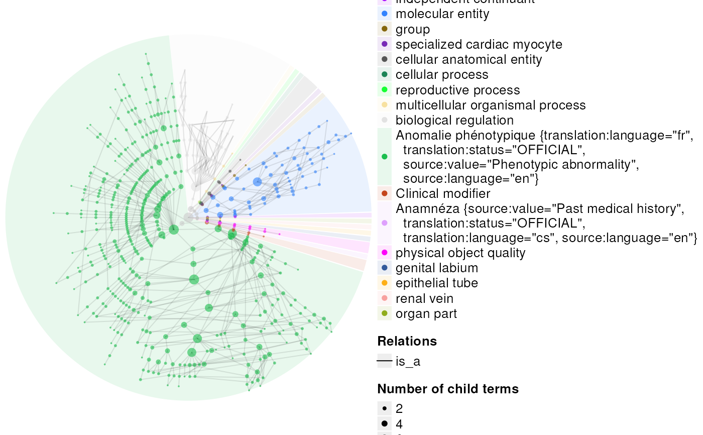
res <- plot_ontology(ont,
terms=100,
types="circular",
partition_by_level=2,
edge_transparency=.9)
#> Randomly sampling 100 term(s).
#> Loading required namespace: DiagrammeR
#> converting DAG to a tree...
#>
#> going through 506 / 506 nodes ... Done.
#> calculating term positions on the DAG...
#>
#> going through 506 / 506 nodes ... Done.
#> making plot...
#> adding links...
#> adding terms...
 #> Best device size: 9.85 x 6.67 inches.
ont <- get_ontology("hp", terms=2)
#> Using cached ontology file (1/1):
#> /github/home/.cache/R/KGExplorer/ontologies/github/hp_v2025-11-24.rds
#> Randomly sampling 2 term(s).
hm <- plot_ontology_heatmap(ont)
#> Adding ancestor metadata.
#> Ancestor metadata already present. Use force_new=TRUE to overwrite.
#> Creating heatmap: ComplexHeatmap
#> Using palette: okabe
#> Using palette: stepped2
#> Using palette: okabe
#> Using palette: watlington
#> Using palette: stepped3
#> Using palette: tableau20
#> Translating ontology terms to ids.
#> term_sim_method: Sim_WP_1994
#> collecting all ancestors of input terms ...
#>
#> going through 0 / 17 ancestors ...
#>
#> going through 17 / 17 ancestors ... Done.
#> collecting all ancestors of input terms ...
#>
#> going through 0 / 17 ancestors ...
#>
#> going through 17 / 17 ancestors ... Done.
#> Converted ontology to: similarity
#> Saving plot --> /tmp/RtmpcvQwaB/file60336dbe0f72plot_ontology_heatmap.pdf
#> Best device size: 9.85 x 6.67 inches.
ont <- get_ontology("hp", terms=2)
#> Using cached ontology file (1/1):
#> /github/home/.cache/R/KGExplorer/ontologies/github/hp_v2025-11-24.rds
#> Randomly sampling 2 term(s).
hm <- plot_ontology_heatmap(ont)
#> Adding ancestor metadata.
#> Ancestor metadata already present. Use force_new=TRUE to overwrite.
#> Creating heatmap: ComplexHeatmap
#> Using palette: okabe
#> Using palette: stepped2
#> Using palette: okabe
#> Using palette: watlington
#> Using palette: stepped3
#> Using palette: tableau20
#> Translating ontology terms to ids.
#> term_sim_method: Sim_WP_1994
#> collecting all ancestors of input terms ...
#>
#> going through 0 / 17 ancestors ...
#>
#> going through 17 / 17 ancestors ... Done.
#> collecting all ancestors of input terms ...
#>
#> going through 0 / 17 ancestors ...
#>
#> going through 17 / 17 ancestors ... Done.
#> Converted ontology to: similarity
#> Saving plot --> /tmp/RtmpcvQwaB/file60336dbe0f72plot_ontology_heatmap.pdf